BioCro module functions

BioCro modules are named sets of equations, and each module is available from a BioCro module library. Each module is identified by a fully-qualified name that includes the name of its library and its local name within that library. The functions here provide ways to access information about modules and to calculate their output values from sets of input values.

module_info returns essential information about a BioCro module.

quantity_list_from_names initializes a list of named numeric elements from a set of names.

evaluate_module runs a BioCro module using a list of input quantity values.

module_response_curve runs a BioCro module repeatedly with different input quantity values to produce a response curve.

Usage

module_info(module_name, verbose = TRUE)

  quantity_list_from_names(quantity_names)

  evaluate_module(module_name, input_quantities)

  module_response_curve(module_name, fixed_quantities, varying_quantities)

Arguments

module_name: A string specifying one BioCro module, formatted like library_name:local_module_name, where library_name is the name of a library that contains a module with local name local_module_name; such fully-qualified module names can be formed manually or with module_paste.
verbose: A boolean indicating whether or not to print information to the R console.
input_quantities: A list of named numeric elements representing the input quantities required by the module; any extraneous quantities will be ignored by the module.
quantity_names: A vector of strings.
fixed_quantities: A list of named numeric elements representing input quantities required by the module whose values should be considered to be constant; any extraneous quantities will be ignored by the module.
varying_quantities: A data frame where each column represents an input quantity required by the module whose value varies across the response curve.

Details

By providing avenues for retrieving information about a module and evaluating a module's equations, the module_info and evaluate_module functions form the main interface to individual BioCro modules from within R. The quantity_list_from_names function is a convenience function for preparing suitable quantity lists to pass to evaluate_module.

The module_response_curve function provides a convenient way to calculate a module response curve. To do this, a user must specify a module to use, the values of any fixed input quantities (input_quantities), and a sequence of values for other quantities that vary across the response curve (varying_quantities). The returned data frame includes all the information that would be required to reproduce the curve: the full-qualified module name, all inputs (including ones with constant values), and the outputs. Note: if one quantity q is both an input and output of the module, its input value will be stored in the q column of the returned data frame and its output value will be stored in the q.1 column; this renaming is performed automatically by the make.unique function.

Value

module_info

An invisible list of several named elements containing essential information about the module:

module_name: The module's (not-fully-qualified) name
inputs: A character vector of the module's inputs
outputs: A character vector of the module's outputs
type: The module's type represented as a string (either 'differential' or 'direct')
euler_requirement: Indicates whether the module requires a fixed-step Euler ODE solver when used in a BioCro simulation
creation_error_message: Describes any errors that occurred while creating an instance of the module

quantity_list_from_names

A list of named numeric elements, where the names are set by quantity_names and each value is set to 1.

evaluate_module

A list of named numeric elements representing the values of the module's outputs as calculated from the input_quantities according to the module's equations.

module_response_curve

A data frame where the first column is the fully-qualified name of the module that produced the response curve and the remaining columns are the module's input and output quantities. Each row corresponds to a row in the varying_quantities.

Examples

# Example 1: printing information about the 'BioCro' module library's
# 'c3_assimilation' module to the R console
module_info('BioCro:c3_assimilation')
#> 
#> 
#> Module name:
#>   c3_assimilation
#> 
#> Module input quantities:
#>   Qabs
#>   Tleaf
#>   temp
#>   rh
#>   vmax1
#>   jmax
#>   tpu_rate_max
#>   Rd
#>   b0
#>   b1
#>   Gs_min
#>   Catm
#>   atmospheric_pressure
#>   O2
#>   theta
#>   StomataWS
#>   electrons_per_carboxylation
#>   electrons_per_oxygenation
#>   beta_PSII
#>   gbw
#> 
#> Module output quantities:
#>   Assim
#>   Gs
#>   Cs
#>   RHs
#>   Ci
#>   GrossAssim
#>   Assim_conductance
#>   Rp
#>   iterations
#> 
#> Module type (differential or direct):
#>   direct
#> 
#> Requires a fixed step size Euler ode_solver:
#>   no
#> 

# Example 2: getting the inputs to the 'BioCro' module library's
# 'thermal_time_linear' module, generating a default input list, and using it to
# run the module
info <- module_info('BioCro:thermal_time_linear', verbose = FALSE)
inputs <- quantity_list_from_names(info$inputs) # All inputs will be set to 1
outputs <- evaluate_module('BioCro:thermal_time_linear', inputs)

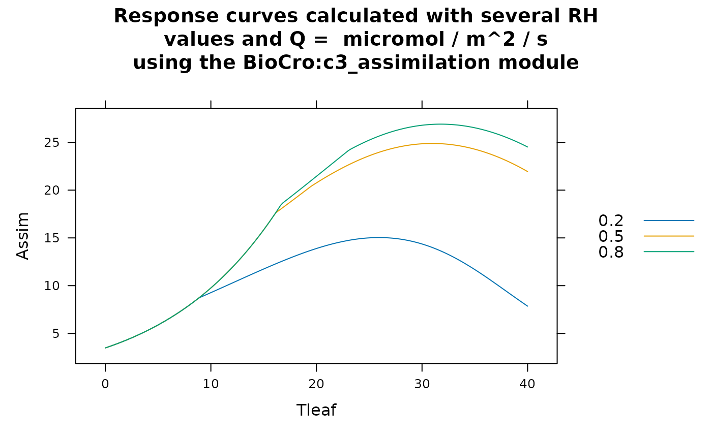
# Example 3: calculating the temperature response of light saturated net
# assimilation at several values of relative humidity in the absence of water
# stress using the 'BioCro' module library's 'c3_assimilation' module and
# the default soybean parameters. Here, the leaf temperature and humidity values
# are independent of each other, so we use the `expand.grid` function to form a
# data frame of all possible combinations of their values. Then we set the
# ambient temperature equal to the leaf temperature.
rc <- module_response_curve(
  'BioCro:c3_assimilation',
  within(soybean$parameters, {Qabs = 2000; StomataWS = 1; gbw = 1.2}),
  within(
    expand.grid(
      Tleaf = seq(from = 0, to = 40, length.out = 201),
      rh = c(0.2, 0.5, 0.8)
    ),
    {temp = Tleaf}
  )
)

caption <- paste(
  "Response curves calculated with several RH\nvalues and Q =",
  unique(rc$Qp),
  "micromol / m^2 / s\nusing the",
  unique(rc$module_name),
  "module"
)

lattice::xyplot(
  Assim ~ Tleaf,
  group = rh,
  data = rc,
  auto = TRUE,
  type = 'l',
  main = caption
)

Usage

Arguments

Details

Value

See also

Examples