Using the Ball-Berry Model in Crop Growth Simulations
Source:vignettes/web_only/ball_berry_model.Rmd
ball_berry_model.Rmd1 Overview
The Ball-Berry is a simple empirical model for the steady-state response of stomata to external conditions and was first described in Ball et al. (1987). The main idea is that stomata open in response to brighter light or low CO\(_2\) availability, and close in response to low humidity (to limit water losses from transpiration). This idea can be expressed mathematically as
\[\begin{equation} g_{sw} = b_0 + b_1 \cdot \frac{ A_n \cdot h_s}{C_s} \quad \text{if} \; A_n \geq 0, \tag{1.1} \end{equation}\]
where \(g_{sw}\) is the stomatal conductance to water vapor diffusion, \(A_n\) is the net CO\(_2\) assimilation rate, \(b_0\) and \(b_1\) are the Ball-Berry intercept and slope, \(h_s\) is the relative humidity at the leaf surface, and \(C_s\) is the CO\(_2\) concentration at the leaf surface. When \(A_n < 0\), \(g_{sw} = b_0\). Here, the net assimilation is a proxy for the incident light intensity and captures the nonlinear response of \(g_{sw}\) to light. The quantity \(A_n \cdot h_s / C_s\) is often called the Ball-Berry index; thus, the model states that stomatal conductance is a linear function of the Ball-Berry index, and the model is parameterized by the Ball-Berry slope and intercept.
Several critiques of this model have been made, and other models of stomatal response exist (Tardieu and Davies 1993; Leuning 1995; Dewar 2002). Nevertheless, the Ball-Berry model remains widely-used due to its simplicity. (However, as we will see in the following section, it is not always so simple to use in the context of crop growth modeling!)
2 Using the Model for Crop Growth Modeling
There are several complexities associated with using this equation for crop growth modeling. One is that \(A_n\) depends on the CO\(_2\) concentration inside the leaf, so combined models employing the Ball-Berry equation and mechanistic equations for photosynthesis must generally be solved iteratively. Another complexity associated with crop growth modeling is that the CO\(_2\) and H\(_2\)O concentrations at the leaf surface are not usually known beforehand. Instead, they must be determined from the ambient values, boundary layer conductances, and fluxes using one-dimensional gas flow equations of the form \(F = g \cdot (c_2 - c_1)\), where \(F\) is a flux, \(g\) is a conductance, and \(c_1\) and \(c_2\) are gas concentrations at two physical locations. The remainder of this section will describe how these gas flow equations can be used to determine \(C_s\) and \(h_s\).
2.1 Determining \(C_s\)
Assuming steady-state conditions, the CO\(_2\) flux across the boundary layer is given by \(A_n\), allowing us to find \(C_s\) using a single gas flow equation:
\[\begin{equation} C_s = C_a - \frac{A_n}{g_{bc}} = C_a - \frac{A_n \cdot 1.37}{g_{bw}}, \tag{2.1} \end{equation}\]
where \(C_a\) is the ambient CO\(_2\) concentration, \(g_{bc}\) is the boundary layer conductance to CO\(_2\) diffusion, and \(g_{bw}\) is the boundary layer conductance to water vapor diffusion. The two conductances are related by the ratio of diffusivities of CO\(_2\) and H\(_2\)O in the boundary layer, which is typically taken to be 1.37. (For more information about this ratio and its value, see the discussion following Equation B16 in Caemmerer and Farquhar (1981).)
2.2 Determining \(h_s\)
The situation with water vapor is more complicated. The first point is that water vapor flows along concentration gradients, not relative humidity gradients. Concentrations and relative humidities are related by
\[\begin{equation} h = P_w / P_{w,sat}(T) = w \cdot P_{tot} / P_{w,sat}(T), \tag{2.2} \end{equation}\]
where \(h\) is the relative humidity, \(w\) is the water vapor concentration, \(P_w\) is the partial pressure of water vapor, \(P_{w,sat}(T)\) is the saturation water vapor pressure corresponding to the air temperature \(T\), and \(P_{tot}\) is the total gas pressure. The second point is that the water vapor flux \(E\) is initially unknown; instead, we assume that water vapor is fully saturated within the leaf and that the water vapor flow has reached steady-state conditions.
Thus, we can begin with two gas flow equations corresponding to water vapor flux across the boundary layer and stomata (\(E_b\) and \(E_s\), respectively):
\[\begin{equation} E_b = g_{bw} \cdot (w_s - w_a) \tag{2.3} \end{equation}\]
and
\[\begin{equation} E_s = g_{sw} \cdot (w_i - w_s), \tag{2.4} \end{equation}\]
where \(w_a\), \(w_s\), and \(w_i\) are the water vapor concentrations in the ambient air, at the leaf surface, and in the leaf interior, respectively. Note that Equation (2.2) can be used to re-express these concentrations using the corresponding relative humidities (\(h_a\), \(h_s\), and \(h_i\)) and air temperatures (\(T_a\), \(T_s\), and \(T_i\)) at the same locations as follows:
\[\begin{align} w_a &= h_a \cdot \frac{P_{w,sat}(T_a)}{P_{tot}} \\ w_s &= h_s \cdot \frac{P_{w,sat}(T_s)}{P_{tot}} \\ w_i &= h_i \cdot \frac{P_{w,sat}(T_i)}{P_{tot}} = \frac{P_{w,sat}(T_i)}{P_{tot}}, \tag{2.5} \end{align}\]
where we have set \(h_i = 1\) in the latter to reflect the assumption that water vapor is saturated inside the leaf. The leaf’s surface and its interior spaces are assumed to have the same temperature and hence the same saturation water vapor pressure, so we can also set
\[\begin{equation} T_s = T_i = T_l, \tag{2.6} \end{equation}\]
where \(T_l\) is the leaf temperature.
Now, we can replace \(g_{sw}\) in Equation (2.4) with the expression from Equation (1.1), replace the water vapor concentrations and temperatures in Equations (2.3) and (2.4) with the expressions from Equations (2.5) and (2.6), and equate the two fluxes in Equations (2.3) and (2.4) since they must be equal under steady-state conditions. Putting this all together, we can write
\[\begin{equation} \frac{g_{bw}}{P_{tot}} \cdot \big[ h_s \cdot P_{w,sat}(T_l) - h_a \cdot P_{w,sat}(T_a) \big] = \frac{P_{w,sat}(T_l)}{P_{tot}} \cdot \left[ b_0 + b_1 \cdot \frac{A_n \cdot h_s}{C_s} \right] \cdot \left( 1 - h_s \right). \tag{2.7} \end{equation}\]
When multiplied out and regrouped, Equation (2.7) becomes a quadratic equation for \(h_s\):
\[\begin{equation} h_s^2 \cdot \left( b_1 \cdot \frac{A_n}{C_s} \right) + h_s \cdot \left( b_0 + g_{bw} - b_1 \cdot \frac{A_n}{C_s} \right) - \left( g_{bw} \cdot h_a \cdot \frac{P_{w,sat}(T_a)}{P_{w,sat}(T_l)} + b_0 \right) = 0. \tag{2.8} \end{equation}\]
Equation (2.8) can be solved for \(h_s\) using the quadratic formula:
\[\begin{align} h_s &= \frac{-b \pm \sqrt{b^2 - 4 \cdot a \cdot c}}{2 \cdot a}, \\ a &= b_1 \cdot \frac{A_n}{C_s}, \\ b &= b_0 + g_{bw} - b_1 \cdot \frac{A_n}{C_s}, \\ c &= - \left( g_{bw} \cdot h_a \cdot \frac{P_{w,sat}(T_a)}{P_{w,sat}(T_l)} + b_0 \right). \tag{2.9} \end{align}\]
Note that with our assumptions, \(a \geq 0\) and \(c \leq 0\). Thus, \(b^2 - 4 \cdot a \cdot c \geq b^2\), and the \(\sqrt{b^2 - 4 \cdot a \cdot c}\) term in Equation (2.9) is always larger than (or equal to) \(|b|\). Thus, the “minus” root corresponds to a phyically-impossible negative value for \(h_s\), and we always choose the “plus” root
\[\begin{equation} h_s = \frac{-b + \sqrt{b^2 - 4 \cdot a \cdot c}}{2 \cdot a}. \tag{2.10} \end{equation}\]
2.2.1 Dew
If the leaf temperature is lower than the ambient air temperature, it is possible for the water vapor concentration at the leaf surface to exceed the saturation water vapor pressure at the leaf temperature. This would result in \(h_s > 1\), which is not possible. This outcome indicates that water vapor would have condensed on the leaf surface; in other words, that dew would have formed.
3 BioCro Implementation
In BioCro, the Ball-Berry model is implemented by the ball_berry_gs() C++
function, which calculates \(C_s\), \(h_s\), and \(g_{sw}\) with Equations
(2.1), (2.10), and (1.1). We do not have a way to deal with
dew formation in BioCro at the moment, so \(h_s \leq 1\) is forced in the code.
This function can be accessed via the BioCro:ball_berry module.
The model also plays a key role in several other functions and modules that call
ball_berry_gs():
The
c3photoC()C++ function couples the Ball-Berry model with the Farquhar-von-Caemmerer-Berry model for C3 photosynthesis to determine \(A_n\) and \(g_{sw}\) from environmental conditions. This function can be accessed via theBioCro:c3_assimilationmodule. See the module documentation for more information.The
BioCro:c3_leaf_photosynthesismodule couples the Ball-Berry model, the Farquhar-von-Caemmerer-Berry model for C3 photosynthesis, and the Penman-Monteith approach to energy balance to determine \(A_n\), \(g_{sw}\), and \(T_l\) from environmental conditions. See the module documentation for more information.The
c3CanAC()C++ function applies the fully-coupled model used by theBioCro:c3_leaf_photosynthesismodule to sunlit and shaded leaves within a crop canopy to calculate canopy-level photosynthesis. This function can be accessed via theBioCro:c3_canopyandBioCro:ten_layer_c3_canopymodules. See the module documentation for more information.The
c4photoC()C++ function couples the Ball-Berry model with the Collatz model for C4 photosynthesis to determine \(A_n\) and \(g_{sw}\) from environmental conditions. This function can be accessed via theBioCro:c4_assimilationmodule. See the module documentation for more information.The
BioCro:c4_leaf_photosynthesismodule couples the Ball-Berry model, the Collatz model for C3 photosynthesis, and the Penman-Monteith approach to energy balance to determine \(A_n\), \(g_{sw}\), and \(T_l\) from environmental conditions. See the module documentation for more information.The
CanAC()C++ function applies the fully-coupled model used by theBioCro:c4_leaf_photosynthesismodule to sunlit and shaded leaves within a crop canopy to calculate canopy-level photosynthesis. This function can be accessed via theBioCro:c4_canopyandBioCro:ten_layer_c4_canopymodules. See the module documentation for more information.
4 BioCro Examples
Here we will show how BioCro can be used to evaluate the Ball-Berry model or use
it in conjunction with other models of varying complexity. To start, we will
need to load the BioCro and lattice libraries:
4.1 Ball-Berry
Here we will visualize the Ball-Berry model’s output for soybean leaves with several different values of \(A_n\) and \(T_a\). We can see that \(g_{sw}\) and \(h_s\) change with ambient temperature (Figures 4.1 and 4.2) while \(C_s\) does not (Figure 4.3).
# Choose a leaf temperature
Tleaf = 25 # degrees C

# Run the model for different An and Tambient
bb_rc <- module_response_curve(
  'BioCro:ball_berry',
  within(soybean$parameters, {
    gbw = 1.2                # mol / m^2 / s
    leaf_temperature = Tleaf # degress C
    rh = 0.7                 # dimensionless
  }),
  expand.grid(
    net_assimilation_rate = seq(-5, 40, length.out = 201), # micromol / m^2 / s
    temp = seq(Tleaf - 6, Tleaf + 6, by = 2)               # degrees C
  )
)
# Plot gsw
xyplot(
    leaf_stomatal_conductance ~ net_assimilation_rate,
    group = temp,
    data = bb_rc,
    type = 'l',
    auto.key = list(space = 'right'),
    grid = TRUE,
    xlab = "An (micromol / m^2 / s)",
    ylab = "Stomatal conductance (mol / m^2 / s)",
    main = paste(
        "Ball-Berry model with T_leaf =", Tleaf,
        "\nand different T_ambient"
    )
)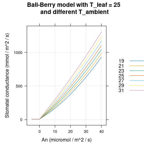
Figure 4.1: \(g_{sw}\) vs \(A_n\) for several different \(T_a\) as predicted by the Ball-Berry model with soybean parameter values.
# Plot hs
xyplot(
    hs ~ net_assimilation_rate,
    group = temp,
    data = bb_rc,
    type = 'l',
    auto.key = list(space = 'right'),
    grid = TRUE,
    xlab = "An (micromol / m^2 / s)",
    ylab = "Relative humidity at leaf surface (dimensionless)",
    main = paste(
        "Ball-Berry model with T_leaf =", Tleaf,
        "\nand different T_ambient"
    )
)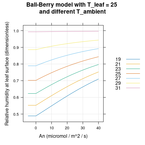
Figure 4.2: \(h_s\) vs \(A_n\) for several different \(T_a\) as predicted by the Ball-Berry model with soybean parameter values.
# Plot cs
xyplot(
    cs ~ net_assimilation_rate,
    group = temp,
    data = bb_rc,
    type = 'l',
    auto.key = list(space = 'right'),
    grid = TRUE,
    xlab = "An (micromol / m^2 / s)",
    ylab = "CO2 concentration at leaf surface (micromol / mol)",
    main = paste(
        "Ball-Berry model with T_leaf =", Tleaf,
        "\nand different T_ambient"
    )
)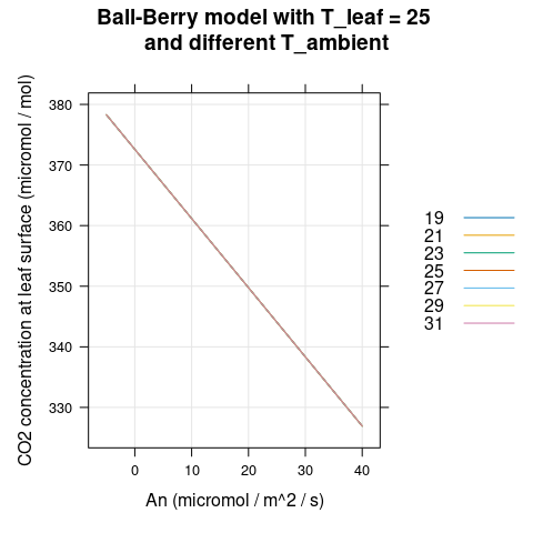
Figure 4.3: \(C_s\) vs \(A_n\) for several different \(T_a\) as predicted by the Ball-Berry model with soybean parameter values.
4.2 Ball-Berry and C3 Photosynthesis
Here we will calculate the response of \(g_{sw}\) and \(A_n\) to the absorbed
quantum photon flux (\(Q_{abs}\)) and ambient humidity in a coupled model
incorporating the Ball-Berry and Farquhar-von-Caemmerer-Berry (FvCB) models.
Although this coupled model also gives us the option to reduce a crop’s
“inherent” Ball-Berry parameters in response to water stress, for this
simulation we will ignore water stress by setting StomataWS = 1. From these
calculations, we can see that the stomatal conductance increases for higher
humidities (Figure 4.4), and that both \(A_n\) and \(g_{sw}\) reach
plateaus at high light levels (Figures 4.4 and
4.5).
# Run the model for different Qabs and rh
lrc <- module_response_curve(
  'BioCro:c3_assimilation',
  within(soybean$parameters, {
    StomataWS = 1 # dimensionless
    Tleaf = 30    # degrees C
    gbw = 1.2     # mol / m^2 / s
    temp = 28     # degrees C
  }),
  expand.grid(
    Qabs = seq(0, 1000, by = 5), # micromol / m^2 / s
    rh = c(0.2, 0.4, 0.6, 0.8)   # dimensionless
  )
)
# Plot gsw
xyplot(
    Gs ~ Qabs,
    group = rh,
    data = lrc,
    type = 'l',
    auto.key = list(space = 'right'),
    grid = TRUE,
    xlab = "Absorbed PPFD (micromol / m^2 / s)",
    ylab = "Stomatal conductance to H2O (mol / m^2 / s)",
    main = "Ball-Berry + FvCB models for\ndifferent humidities"
)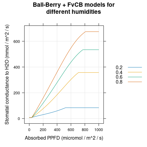
Figure 4.4: \(g_{sw}\) vs \(Q_{abs}\) for several different \(h_a\) as predicted by the coupled Ball-Berry + FvCB model with soybean parameter values.
# Plot An
xyplot(
    Assim ~ Qabs,
    group = rh,
    data = lrc,
    type = 'l',
    auto.key = list(space = 'right'),
    grid = TRUE,
    xlab = "Absorbed PPFD (micromol / m^2 / s)",
    ylab = "Net CO2 assimilation rate (micromol / m^2 / s)",
    main = "Ball-Berry + FvCB models for\ndifferent humidities"
)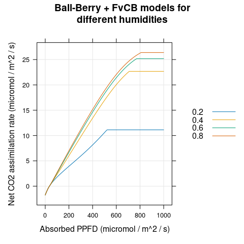
Figure 4.5: \(A_n\) vs \(Q_{abs}\) for several different \(h_a\) as predicted by the coupled Ball-Berry + FvCB model with soybean parameter values.
4.3 Simulated C3 CO\(_2\) Response Curves
Here we can simulate CO\(_2\) response curves at different humidity levels by coupling the Ball-Berry and Farquhar-von-Caemmerer-Berry models to an energy balance equation. Here we will keep the ambient temperature fixed while increasing the ambient CO\(_2\) concentration, as can be done in a gas exchange measurement system like the Licor LI-6800. The environmental conditions will determine \(g_{sw}\), \(A_n\), \(T_l\), and \(C_i\) for each value of \(C_a\), and plots can be generated from these values. In this model, height and windspeed will determine the boundary layer conductance; we choose a large wind speed to ensure high conductance, as would occur in a measurement chamber.
From these calculations:
We can see that \(g_{sw}\) changes with \(C_i\) and \(h_a\) (Figure 4.6), but \(A_n\) plotted against \(C_i\) is the same for all humidities (Figure 4.7). This demonstrates that an A-Ci curve reveals the response of photosynthesis to CO\(_2\) without any influence from the stomata. (Sometimes this idea is expressed by saying that an A-Ci curve “peels away the epidermis.”)
We can also see that the value of \(C_i\) corresponding to each \(C_a\) does depend on the humidity, with higher humidity corresponding to higher \(C_i\) (Figure 4.9). This relationship is mediated by the stomata, which open more in response to higher humidity. Thus, although humidity does not impact the shape of an A-Ci curve, it can have an effect on the range of achievable \(C_i\) values.
The stomatal conductance is largest when \(C_i\) is near 250 ppm, and the leaf temperature is lowest in this range (Figures 4.6 and 4.8). This occurs because the open stomata facilitate evaporative cooling; the cooling effect is stronger at lower humidities where the transpiration rate is higher.
# Set the absorbed photosynthetically active light (in micromol / m^2 / s)
absorbed_ppfd <- 1000

# Determine the total absorbed shortwave light energy (in J / m^2 / s)
absorbed_shortwave <-
    absorbed_ppfd * soybean$parameters$par_energy_content /
        soybean$parameters$par_energy_fraction

# Set the air temperature
air_temperature = 30

# Determine the absorbed longwave light energy (in J / m^2 / s)
absorbed_longwave <- evaluate_module(
    'BioCro:stefan_boltzmann_longwave',
    list(temp = air_temperature, emissivity_sky = 1)
)$absorbed_longwave

aci <- module_response_curve(
    'BioCro:c3_leaf_photosynthesis',
    within(soybean$parameters, {
        StomataWS = 1          # dimensionless
        temp = air_temperature # degrees C
        windspeed = 3          # m / s
        height = 0.8           # m
        gbw_canopy = 0.2       # m / s
        absorbed_ppfd = absorbed_ppfd
        absorbed_shortwave = absorbed_shortwave
        absorbed_longwave = absorbed_longwave
    }),
    expand.grid(
        Catm = seq(100, 1800, by = 5), # micromol / mol
        rh = c(0.4, 0.6, 0.8)          # dimensionless
    )
)
# Plot the gsw-Ci curves
xyplot(
    Gs ~ Ci,
    group = rh,
    data = aci,
    type = 'l',
    auto.key = list(space = 'right'),
    grid = TRUE,
    xlab = 'Intercellular CO2 concentration (micromol / mol)',
    ylab = 'Stomatal conductance to H2O (mol / m^2 / s)',
    main = 'Ball-Berry + FvCB + energy balance\nfor different humidities'
)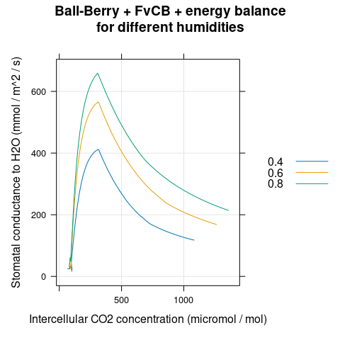
Figure 4.6: \(g_{sw}\) vs \(C_i\) for several different \(h_a\) as predicted by the coupled Ball-Berry + FvCB + energy balance model with soybean parameter values.
# Plot the A-Ci curves
xyplot(
    Assim ~ Ci,
    group = rh,
    data = aci,
    type = 'l',
    auto.key = list(space = 'right'),
    grid = TRUE,
    xlab = 'Intercellular CO2 concentration (micromol / mol)',
    ylab = 'Net CO2 assimilation rate (micromol / m^2 / s)',
    main = 'Ball-Berry + FvCB + energy balance\nfor different humidities'
)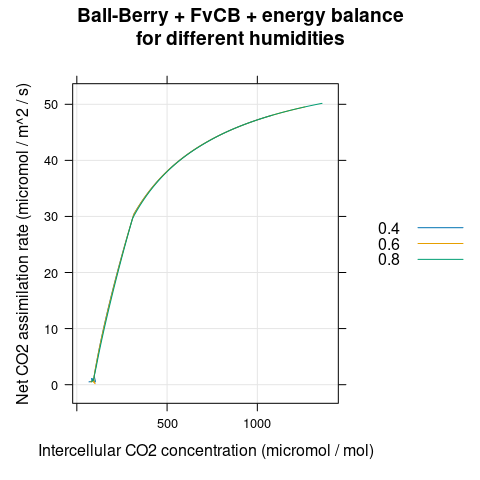
Figure 4.7: \(A_n\) vs \(C_i\) for several different \(h_a\) as predicted by the coupled Ball-Berry + FvCB + energy balance model with soybean parameter values.
# Plot the Tl-Ci curves
xyplot(
    leaf_temperature ~ Ci,
    group = rh,
    data = aci,
    type = 'l',
    auto.key = list(space = 'right'),
    grid = TRUE,
    xlab = 'Intercellular CO2 concentration (micromol / mol)',
    ylab = 'Leaf temperature (degrees C)',
    main = 'Ball-Berry + FvCB + energy balance\nfor different humidities'
)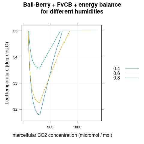
Figure 4.8: \(T_l\) vs \(C_i\) for several different \(h_a\) as predicted by the coupled Ball-Berry + FvCB + energy balance model with soybean parameter values.
# Plot the Ci-Ca curves
xyplot(
    Ci ~ Catm,
    group = rh,
    data = aci,
    type = 'l',
    auto.key = list(space = 'right'),
    grid = TRUE,
    xlab = 'Ambient CO2 concentration (micromol / mol)',
    ylab = 'Intercellular CO2 concentration (micromol / mol)',
    main = 'Ball-Berry + FvCB + energy balance\nfor different humidities'
)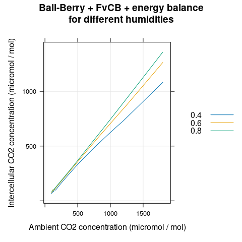
Figure 4.9: \(C_i\) vs \(C_a\) for several different \(h_a\) as predicted by the coupled Ball-Berry + FvCB + energy balance model with soybean parameter values.
4.4 Gas Concentrations Within a C3 Canopy
Here we can see how several quantities change throughout a soybean canopy under a fixed set of environmental conditions when using the fully-coupled Ball-Berry + FvCB + energy balance model for leaf level photosynthesis. For sunlit leaves, we observe the following trends:
The CO\(_2\) concentration at the leaf surface (\(C_s\)) decreases with canopy depth (Figure 4.10).
The relative humidity at the leaf surface (\(C_s\)) increases with canopy depth (Figure 4.11).
The stomatal conductance (\(g_{sw}\)) increases with canopy depth (Figure 4.12).
The leaf temperature (\(T_l\)) generally increases with canopy depth, although the trend is not monotonic (Figure 4.13).
The net assimilation rate (\(A_n\)) decreases with canopy depth (Figure 4.14).
# Run canopy modules
RH_a <- 0.8     # dimensionless; ambient relative humidity
T_ambient <- 30 # degrees C; ambient air temperature
StomataWS <- 1  # no water stress

canres <- run_biocro(
    direct_module_names = c(
        'BioCro:solar_position_michalsky',
        'BioCro:shortwave_atmospheric_scattering',
        'BioCro:incident_shortwave_from_ground_par',
        'BioCro:height_from_lai',
        'BioCro:canopy_gbw_thornley',
        'BioCro:stefan_boltzmann_longwave',
        'BioCro:ten_layer_canopy_properties',
        'BioCro:ten_layer_c3_canopy'
    ),
    parameters = within(soybean$parameters, {
        year = 2022
        time_zone_offset = -6 # CDT
        solar = 1500          # micromol / m^2 / s
        lai = 3               # dimensionless
        rh = RH_a             # dimensionless
        windspeed = 2         # m / s
        temp = T_ambient      # degrees C
        StomataWS = StomataWS # dimensionless
    }),
    drivers = data.frame(fractional_doy = 210.5) # noon on day 210 (July 29 for 2022)
)

# Extract canopy profiles
canopy_profiles_list <- lapply(
    c('sunlit', 'shaded'),
    function(leaf_class) {
        cs_column_names <- grep(
            paste0(leaf_class, '_Cs_layer_[0-9]'),
            colnames(canres),
            value = TRUE
        )

        rhs_column_names <- grep(
            paste0(leaf_class, '_RHs_layer_[0-9]'),
            colnames(canres),
            value = TRUE
        )

        rh_canopy_column_names <- grep(
            paste0(leaf_class, '_RH_canopy_layer_[0-9]'),
            colnames(canres),
            value = TRUE
        )

        gsw_column_names <- grep(
            paste0(leaf_class, '_Gs_layer_[0-9]'),
            colnames(canres),
            value = TRUE
        )

        tl_column_names <- grep(
            paste0(leaf_class, '_leaf_temperature_layer_[0-9]'),
            colnames(canres),
            value = TRUE
        )

        a_column_names <- grep(
            paste0(leaf_class, '_Assim_layer_[0-9]'),
            colnames(canres),
            value = TRUE
        )

        gbw_column_names <- grep(
            paste0(leaf_class, '_gbw_layer_[0-9]'),
            colnames(canres),
            value = TRUE
        )

        data.frame(
            type = leaf_class,
            layer = seq(0, 9),
            Cs = as.numeric(canres[cs_column_names]),
            RHs = as.numeric(canres[rhs_column_names]),
            RH_canopy = as.numeric(canres[rh_canopy_column_names]),
            gsw = as.numeric(canres[gsw_column_names]),
            tl = as.numeric(canres[tl_column_names]),
            A = as.numeric(canres[a_column_names]),
            gbw = as.numeric(canres[gbw_column_names])
        )
    }
)

canopy_profiles <- do.call(rbind, canopy_profiles_list)
# Plot the Cs profiles
xyplot(
    Cs ~ layer,
    group = type,
    data = canopy_profiles,
    type = 'l',
    auto.key = list(space = 'right'),
    grid = TRUE,
    xlab = 'Canopy layer (0 is top, 9 is bottom)',
    ylab = 'CO2 concentration at leaf surface (micromol / mol)',
    main = 'Ball-Berry + FvCB + energy balance\nwithin a soybean canopy'
)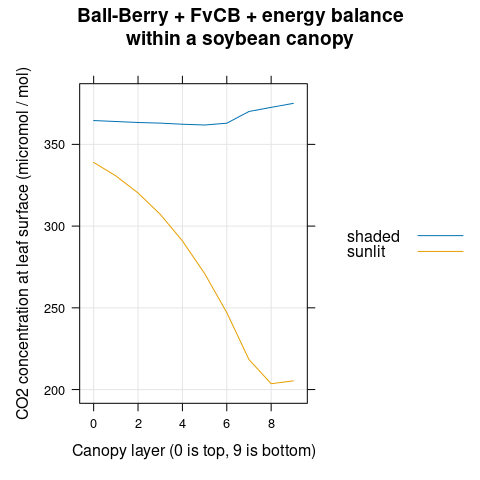
Figure 4.10: \(C_s\) vs canopy layer for sunlit and shaded leaves as predicted by the coupled Ball-Berry + FvCB + energy balance model with soybean parameter values.
# Plot the RHs profiles
xyplot(
    RHs + RH_canopy ~ layer,
    group = type,
    data = canopy_profiles,
    type = 'l',
    auto.key = list(space = 'top'),
    grid = TRUE,
    xlab = 'Canopy layer (0 is top, 9 is bottom)',
    ylab = 'Relative humidity (micromol / mol)',
    main = 'Ball-Berry + FvCB + energy balance\nwithin a soybean canopy'
)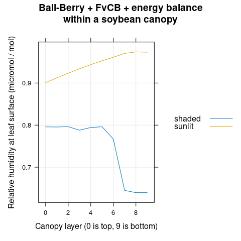
Figure 4.11: Relative humidities at the leaf surface (RHs) and just outside the leaf boundary layer (RH_canopy) plotted against canopy layer for sunlit and shaded leaves as predicted by the coupled Ball-Berry + FvCB + energy balance model with soybean parameter values.
# Plot the gsw profiles
xyplot(
    gsw ~ layer,
    group = type,
    data = canopy_profiles,
    type = 'l',
    auto.key = list(space = 'right'),
    grid = TRUE,
    xlab = 'Canopy layer (0 is top, 9 is bottom)',
    ylab = 'Stomatal conductance to H2O (mol / m^2 / s)',
    main = 'Ball-Berry + FvCB + energy balance\nwithin a soybean canopy'
)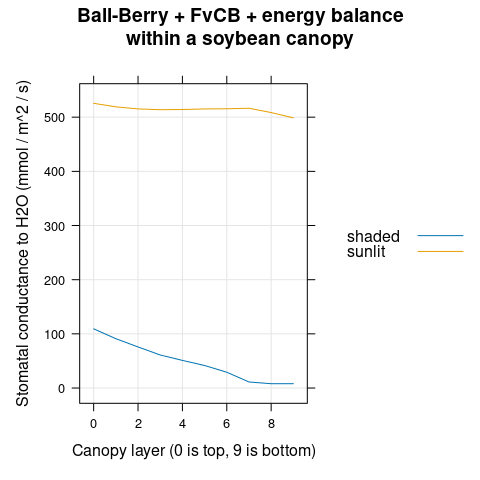
Figure 4.12: \(g_{sw}\) vs canopy layer for sunlit and shaded leaves as predicted by the coupled Ball-Berry + FvCB + energy balance model with soybean parameter values.
# Plot the leaf temperature profiles
xyplot(
    tl ~ layer,
    group = type,
    data = canopy_profiles,
    type = 'l',
    auto.key = list(space = 'right'),
    grid = TRUE,
    xlab = 'Canopy layer (0 is top, 9 is bottom)',
    ylab = 'Leaf temperature (degrees C)',
    main = 'Ball-Berry + FvCB + energy balance\nwithin a soybean canopy'
)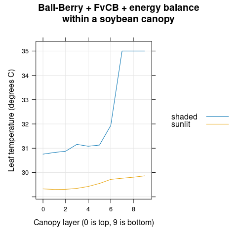
Figure 4.13: \(T_l\) vs canopy layer for sunlit and shaded leaves as predicted by the coupled Ball-Berry + FvCB + energy balance model with soybean parameter values.
# Plot the assimilation profiles
xyplot(
    A ~ layer,
    group = type,
    data = canopy_profiles,
    type = 'l',
    auto.key = list(space = 'right'),
    grid = TRUE,
    xlab = 'Canopy layer (0 is top, 9 is bottom)',
    ylab = 'Net CO2 assimilation rate (micromol / m^2 / s)',
    main = 'Ball-Berry + FvCB + energy balance\nwithin a soybean canopy'
)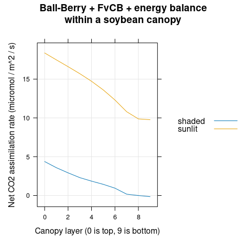
Figure 4.14: \(A_n\) vs canopy layer for sunlit and shaded leaves as predicted by the coupled Ball-Berry + FvCB + energy balance model with soybean parameter values.
# Plot the assimilation profiles
xyplot(
    gbw ~ layer,
    group = type,
    data = canopy_profiles,
    type = 'l',
    auto.key = list(space = 'right'),
    grid = TRUE,
    xlab = 'Canopy layer (0 is top, 9 is bottom)',
    ylab = 'Boundary layer conductance to H2O (mol / m^2 / s)',
    main = 'Ball-Berry + FvCB + energy balance\nwithin a soybean canopy'
)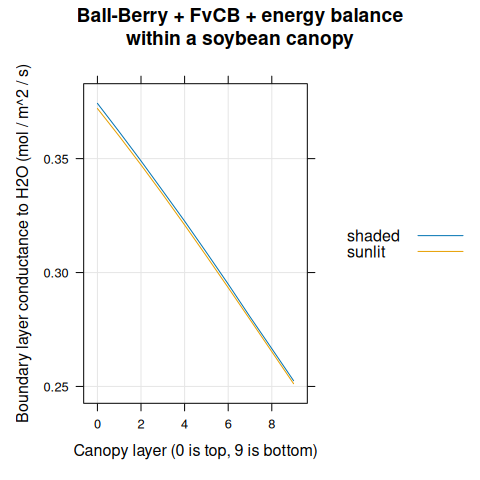
Figure 4.15: \(g_{bw}\) vs canopy layer for sunlit and shaded leaves as predicted by the coupled Ball-Berry + FvCB + energy balance model with soybean parameter values.
4.5 Soybean Modeling
Here we can see how the Ball-Berry slope can affect soybean yield. The slope encapsulates the “willingness” of a crop to open its stomata. When resources are plentiful, higher stomatal conductance may allow for more carbon assimilation and hence growth. On the other hand, higher stomatal conductance increases water losses due to transpiration, and can exacerbate drought stress. Thus, the exact impact of a change in \(b_1\) will therefore strongly depend on the particular location and weather.
In BioCro, the soil water content determines the water stress level in the
plant, reducing the Ball-Berry parameters during times of low water
availability. At the same time, canopy transpiration influences the soil water
content, with higher transpiration rates causing a faster depletion of soil
water. In this example, we will just use weather data from 2002 in Champaign,
Illinois; under these conditions, increasing the Ball-Berry slope causes the
final seed mass (called Grain here) to increase (Figure
4.16).
# Use partial application to create a function that runs a soybean simulation
# for a given value of the Ball-Berry slope
bb1_func <- with(soybean, {partial_run_biocro(
    initial_values,
    parameters,
    soybean_weather[['2002']],
    direct_modules,
    differential_modules,
    ode_solver,
    'b1' # the name of the parameter we wish to vary
)})

# Run the soybean model for several different slope values
bb1_result_list <- lapply(
    seq(soybean$parameters$b1 - 3, soybean$parameters$b1 + 3, by = 1.5),
    function(x) {
        within(bb1_func(x), {b1 = x})
    }
)

# Collect the results into a single data frame
bb1_result <- do.call(rbind, bb1_result_list)
# Plot soybean biomass values for different values of the Ball-Berry slope
xyplot(
    Leaf + Stem + Root + Grain ~ fractional_doy,
    group = b1,
    data = bb1_result,
    type = 'l',
    auto.key = list(space = 'right'),
    grid = TRUE,
    xlab = 'Day of year (2002)',
    ylab = 'Biomass (Mg / ha)',
    main = 'Testing different soybean Ball-Berry slope values'
)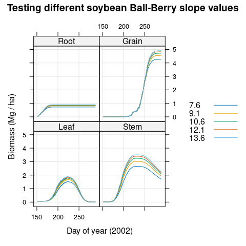
Figure 4.16: Soybean biomass values predicted for Champaign, Illinois during 2002 using different values of the Ball-Berry slope \(b_1\).