Calculate Derivatives for Differential Quantities
system_derivatives.RdSolving a BioCro model using one of R's available differential equation solvers
Arguments
- parameters
Identical to the corresponding argument from
run_biocro.- drivers
Identical to the corresponding argument from
run_biocro.- direct_module_names
Identical to the corresponding argument from
run_biocro.- differential_module_names
Identical to the corresponding argument from
run_biocro.
Details
system_derivatives accepts the same input arguments as
run_biocro with the exceptions of ode_solver and
initial_values; this function is intended to be passed to an ODE solver
in R, which will solve for the system's time dependence as its diffferential
quantities evolve from their initial values, so ode_solver and
initial_values are not required here.
When using one of the pre-defined crop growth models, it may be helpful to
use the with command to pass arguments to system_derivatives;
see the documentation for crop_model_definitions for more
information.
Value
The return value of system_derivatives is a function with three inputs
(t, differential_quantities, and parms) that returns
derivatives for each of the differential quantities in the dynamical system
determined by the original inputs (parameters, drivers,
direct_module_names, and differential_module_names).
This function signature and the requirements for its inputs are set by the
LSODES function from the deSolve package. The t input
should be a single time value and the differential_quantities input
should be a vector with the names of the differential quantities defined by
the modules. parms is required by LSODES, but we don't use it
for anything.
This function can be passed to LSODES as an alternative integration
method, rather than using one of BioCro's built-in solvers.
Examples
# Note: Example 3 below may take several minutes to run. Patience is required!

# Example 1: calculating a single derivative using a soybean model

soybean_system <- system_derivatives(
  soybean$parameters,
  soybean_weather$'2002',
  soybean$direct_modules,
  soybean$differential_modules
)

derivs <- soybean_system(0, unlist(soybean$initial_values), NULL)

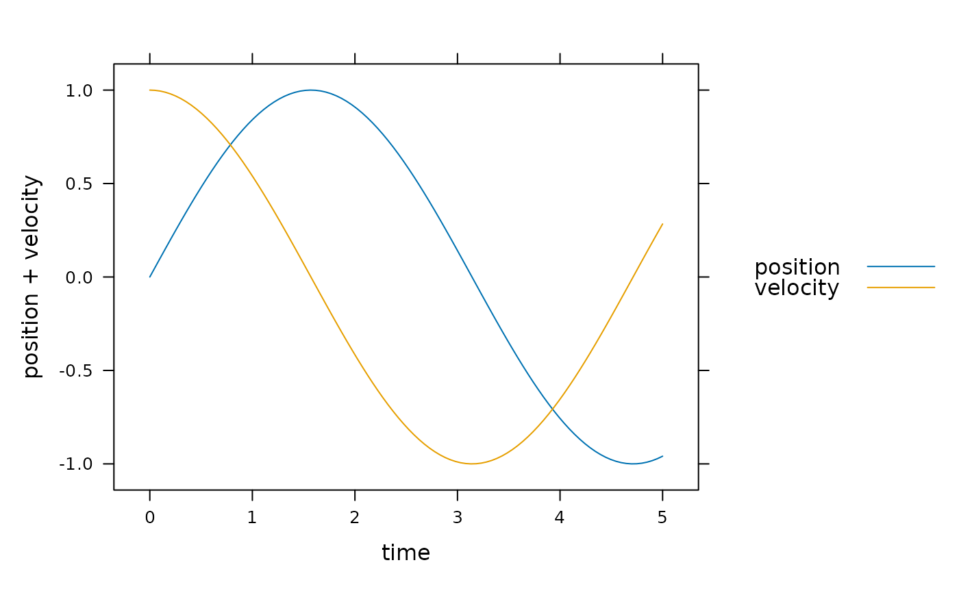
# Example 2: a simple oscillator with only one module

times = seq(0, 5, by = 1) # times spaced by `timestep`

oscillator_system_derivatives <- system_derivatives(
  list(
    timestep = 1,
    mass = 1,
    spring_constant = 1
  ),
  data.frame(time = times),
  c(),
  'BioCro:harmonic_oscillator'
)

result <- as.data.frame(deSolve::lsodes(
  c(position=0, velocity=1),
  times,
  oscillator_system_derivatives
))

lattice::xyplot(
  position + velocity ~ time,
  type='l',
  auto=TRUE,
  data=result
)


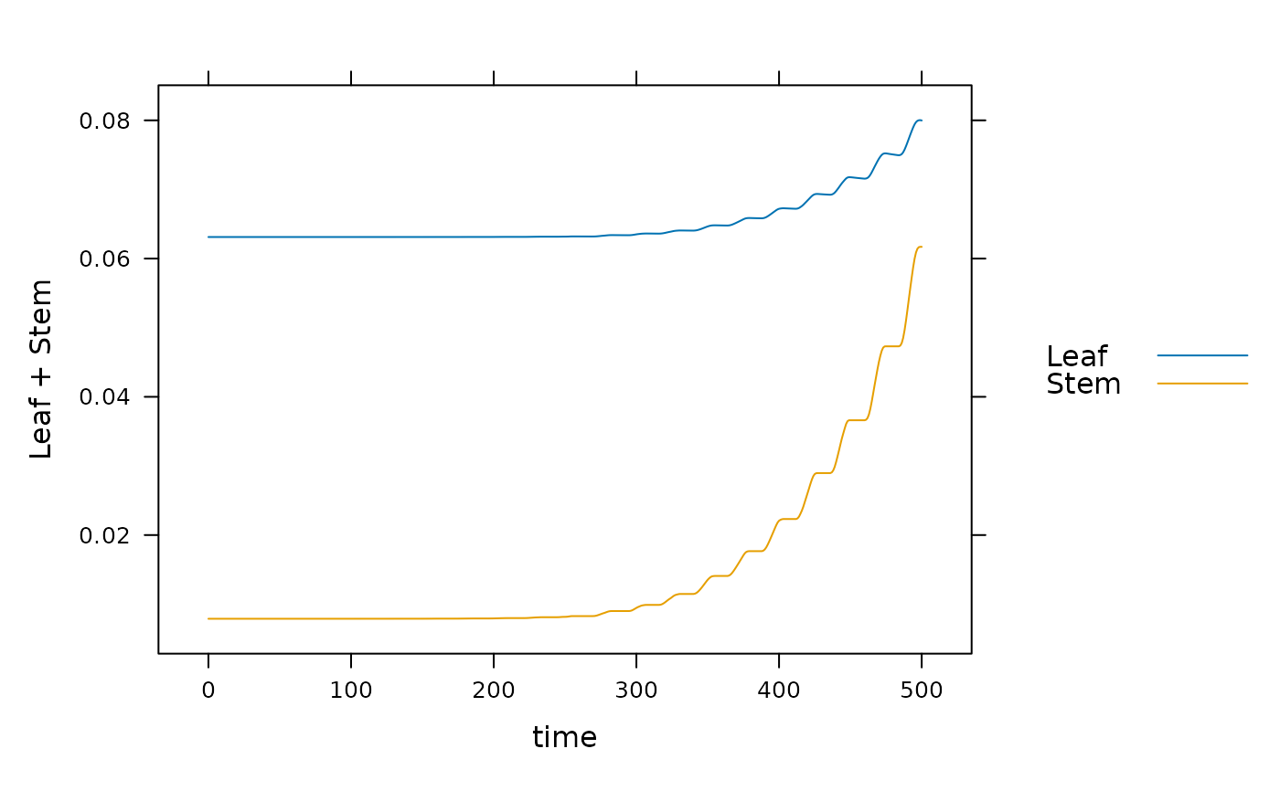
# Example 3: solving 500 hours of a soybean simulation. This will run slowly
# compared to a regular call to `run_biocro`.

# \donttest{

soybean_system <- system_derivatives(
  soybean$parameters,
  soybean_weather$'2002',
  soybean$direct_modules,
  soybean$differential_modules
)

times = seq(from=0, to=500, by=1)

result <- as.data.frame(deSolve::lsodes(unlist(soybean$initial_values), times, soybean_system))

lattice::xyplot(Leaf + Stem ~ time, type='l', auto=TRUE, data=result)

# }
# }